145. Basic properties of ferromagnetics

Though there are not many ferromagnetic bodies in nature, they are the most practical. After all, only they have magnetic properties clearly expressed. In addition, their magnetic properties are much more complex and diverse than those of diaphragmatic and paramagnetic bodies. The nature of ferromagnetism is also much more complex.

We have already mentioned that ferromagnetics are magnetized in the direction of the magnetic field. This brings them closer to the paramagnetics, both \(\mu > 1\). But ferromagnetics \(\mu\) can have many more than one. Finally, ferromagnetic bodies have residual magnetism, which paramagnetic bodies do not.

The magnetic permeability of ferromagnetics is not constant. It depends on the size of the magnetic field. And not only from the magnetic field at a given moment in time, but also from the "history of the sample", that is those fields that acted on the substance in the previous moments of time. We shall stop on it in more details a little later.

At some specific temperature for a given ferromagnetic, the ferromagnetic properties disappear and the substance becomes paramagnetic. This temperature is called the Curie temperature, named after the French scientist Marie Curie who discovered this phenomenon. It is not difficult to detect the existence of the Curie point, at this temperature the residual magnetism disappears and permanent magnets are demagnetized. If strongly to heat up the magnetized nail it will lose ability to attract to itself iron subjects. The Curie temperature is \(753^0 C\) for iron, \(3653^0 C\) for nickel and \(1000^0 C\) for cobalt. There are ferromagnetic alloys that have a Curie temperature below \(100^0 C\).

The magnetic state of ferromagnetics is conveniently characterized by a value called magnetization. If a long homogeneous rod is placed inside a solenoid, the magnetic induction inside it becomes \(B \,= \,\mu\,B_0\). The difference between \(B\) and \(B_0\) can serve as a measure of magnetization of the material. By definition, magnetization \(l\) is equal to

\( l \,= B - B_0 \,= \,(\mu - 1)B_0 \) (13-2)

The dependence of magnitude \(l\) on \(B_0\) is complex, because \(\mu\) for ferromagnetics depends on \(B_0\). The dependence of \(l\) on \(B_0\) shows a so-called magnetization curve, which can be found experimentally (see \(\S 142\)).

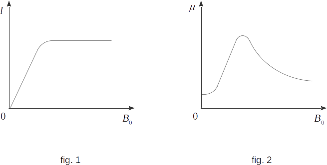
Experience gives us this. If the iron sample was not pre-magnetized, the value of \(l\) initially increases with increasing \(B_0\) almost by linear law (fig. 1). But then, even in relatively weak fields, saturation occurs, the magnetization remains unchanged despite the increase of \(B_0\). Here we can immediately assume that at saturation all elementary currents are oriented completely along the field, so that with further growth of \(B_0\) the field created by them can no longer grow. This is what it really is.

If we plot the dependence \(\mu\) on \(B_0\), we obtain a curve (fig. 2) with a rather complex shape in accordance with dependence \(l(B_0)\) (fig. 1) and equation \((13-2)\). It should be emphasized that each ferromagnetic has its own individual magnetization curve and a curve showing the dependence of m on the magnetizing field.

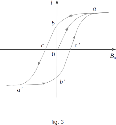
In fact, dependence \(l\) on \(B_0\) is even more complex than shown in figure 1. The point is that this dependency is not straightforward. Magnetization depends not only on the field at the moment, but also on what its value was in the previous moments. We will get the curve shown in figure 1 only if the sample of ferromagnetic was not originally magnetized. If the magnetizing field decreases after reaching saturation, \(l\) will decrease magnetizing more slowly than its growth. This phenomenon is called magnetic hysteresis (which means lag).

The general character of dependence \(l\) on \(B_0\) is shown in figure 3. The line segment \(oa\) represents a magnetization curve similar to that shown in figure 1. At point \(a\), saturation is achieved. When \(B_0\) is reduced to zero, the magnetization is reduced according to the segment of the \(ab\) curve. At \(B_0=0\), the magnetization is different from zero. Its value \(l_r=ob\,\) represents the residual magnetization. The ferromagnetic sample generates a magnetic field without external magnetization. It is therefore a permanent magnet. If the magnetic induction \(B_0\) increases in the opposite direction, the magnetization decreases and only at \(B_{0c}=oc\) it become equal to zero. The value of \(B_{0c}\) is called a coercive (withstand) force. This is the field that should be created to demagnetize the sample. At point \(a'\), the sample is magnetized again until saturation, but in the opposite direction. By reducing the magnetic field to zero and increasing it again until saturation (point \(a\)), we obtain a closed curve symmetrical to point \(o\), called the hysteresis loop.

Different ferromagnetic materials have different forms of hysteresis loop. The shape of the hysteresis loop is the most important magnetic characteristic of the material.

A distinction is made between "soft" and "hard" materials in magnetic terms. A soft material has a small loop area (fig. 4a) and consequently low residual magnetization and coercive force. Such substances include: iron, parmalloy (an alloy of iron and nickel), and etc. A hard material has a large hysteresis loop surface (fig. 4b), the residual magnetization and coercive force are large. Therefore, these materials (including steel and many alloys) are used to produce permanent magnets.

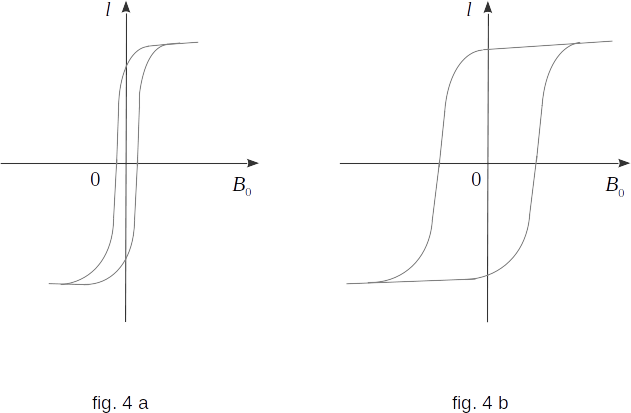
Soft materials are used in the manufacture of transformer cores, electric current generators, electric motors, etc. Under working conditions cores are all the time re-magnetized in variable magnetic fields. Re-magnetization requires work equal in size to the area of the hysteresis loop. (This work is not related to the emission of heat by Foucault currents.) Therefore, in soft materials the energy loss is less than in hard materials.